Getting started
Installation
inference-tools is available from PyPI, so can be easily installed using pip: as follows:
pip install inference-tools
If pip is not available, you can clone from the GitHub source repository or download the files from PyPI directly.
Jupyter notebook demos
In addition to the example code present in the online documentation for each class/function in the package, there is also a set of Jupyter notebook demos which can be found in the /demos/ directory of the source code.
Example - Gaussian peak fitting
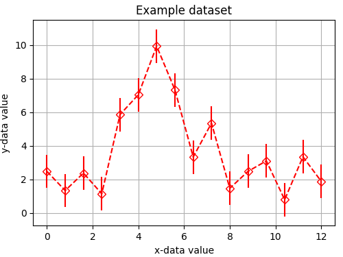
Suppose we have the following dataset:
x_data = [0.00, 0.80, 1.60, 2.40, 3.20, 4.00, 4.80, 5.60,
          6.40, 7.20, 8.00, 8.80, 9.60, 10.4, 11.2, 12.0]

y_data = [2.473, 1.329, 2.370, 1.135, 5.861, 7.045, 9.942, 7.335,
          3.329, 5.348, 1.462, 2.476, 3.096, 0.784, 3.342, 1.877]

y_error = [1., 1., 1., 1., 1., 1., 1., 1.,
           1., 1., 1., 1., 1., 1., 1., 1.]
Our model \(F(x)\) for this data is a Gaussian plus a constant background such that
where our model parameters are the area under the gaussian \(A\), the width \(w\), center \(c\) and background \(b\).
In this example we’re going to:
Construct a likelihood distribution using the model and our dataset.
Construct a prior distribution for the model parameters.
Combine the likelihood and prior to create a posterior distribution.
Sample from the posterior using MCMC.
Use the sample to make inferences about the model parameters.
Constructing the likelihood
The first step is to implement our model. For simple models like this one this can be
done using just a function, but as models become more complex it is becomes useful to
build them as classes. Here we implement the model as the PeakModel class, where by
defining the __call__ instance method, an instance of PeakModel can be called as a
function to return a prediction of the y-data values.
class PeakModel:
    def __init__(self, x_data):
        """
        The __init__ should be used to pass in any data which is required
        by the model to produce predictions of the y-data values.
        """
        self.x = x_data

    def __call__(self, theta):
        return self.forward_model(self.x, theta)

    @staticmethod
    def forward_model(x, theta):
        """
        The forward model must make a prediction of the experimental data we would
        expect to measure given a specific set model parameters 'theta'.
        """
        # unpack the model parameters
        area, width, center, background = theta
        # calculate and return the prediction of the y-data values
        z = (x - center) / width
        gaussian = exp(-0.5 * z**2) / (sqrt(2 * pi) * width)
        return area * gaussian + background
Inference-tools has a variety of likelihood classes which allow you to easily construct a likelihood function given the measured data and your forward-model.
As in this example we assume the errors on the y-data values to be Gaussian, we use the
GaussianLikelihood class from the likelihoods module:
from inference.likelihoods import GaussianLikelihood
likelihood = GaussianLikelihood(
    y_data=y_data,
    sigma=y_error,
    forward_model=PeakModel(x_data)
)
Instances of the likelihood classes can be called as functions, and return the log-likelihood when passed a vector of model parameters.
Constructing the prior
In the common case that the prior distribution for each model variable is independent of
the others (i.e. the prior over all variables can be written as a product of priors over
each individual variable) the inference.priors module has tools which allow us to
build a prior easily.
Which model parameters are assigned to a given prior is specified using the indices of
those parameters (i.e. the position they hold in the parameter vector as defined in the
PeakModel class we wrote earlier).
Suppose we want the area, width and background parameters of the model to each have an
exponential prior. The indices of the area, width and background parameters are
[0, 1, 3] respectively, and we pass these indices to the ExponentialPrior class
via the variable_indices argument:
from inference.priors import ExponentialPrior
exp_prior = ExponentialPrior(beta=[50., 20., 20.], variable_indices=[0, 1, 3])
We can assign the ‘center’ parameter a uniform distribution in the same way using
the UniformPrior class:
from inference.priors import UniformPrior
uni_prior = UniformPrior(lower=0., upper=12., variable_indices=[2])
Now we use the JointPrior class to combine the various components into a single prior
distribution which covers all the model parameters:
from inference.priors import JointPrior
prior_components = [exp_prior, uni_prior]
prior = JointPrior(components=prior_components, n_variables=4)
Sampling from the posterior
The likelihood and prior can be easily combined into a posterior distribution
using the Posterior class:
from inference.posterior import Posterior
posterior = Posterior(likelihood=likelihood, prior=prior)
Now we have constructed a posterior distribution, we can sample from it using Markov-chain Monte-Carlo (MCMC).
The inference.mcmc module contains implementations of various MCMC sampling algorithms.
Here we import the PcaChain class and use it to create a Markov-chain object:
from inference.mcmc import PcaChain
chain = PcaChain(posterior=posterior, start=initial_guess)
We generate samples by advancing the chain by a chosen number of steps using the advance method:
chain.advance(25000)
We can check the status of the chain using the plot_diagnostics method:
chain.plot_diagnostics()
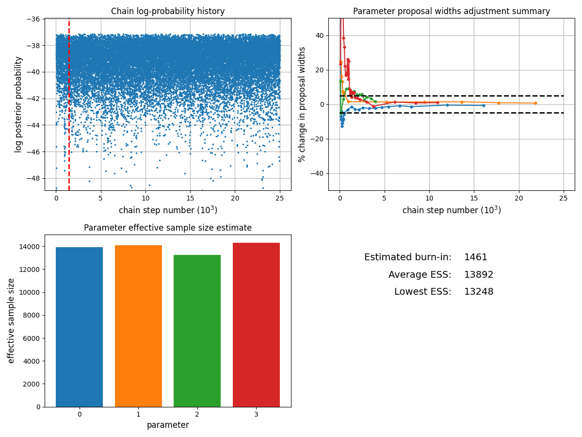
The burn-in (how many samples from the start of the chain are discarded) can be passed as an argument to methods which access or plot sampling results:
burn = 5000
Using the sample to infer the model parameters
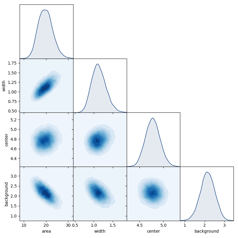
We can get a overview of the posterior using the matrix_plot method
of chain objects, which plots all possible 1D & 2D marginal distributions
of the full parameter set (or a chosen sub-set).
labels = ['area', 'width', 'center', 'background']
chain.matrix_plot(labels=labels, burn=burn)
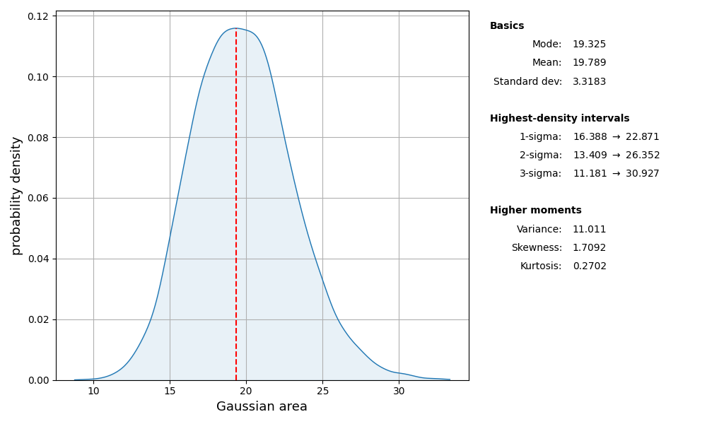
We can easily estimate 1D marginal distributions for any parameter
using the get_marginal method:
area_pdf = chain.get_marginal(0, burn=burn)
area_pdf.plot_summary(label='Gaussian area')
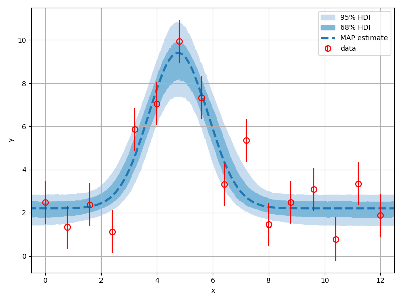
We can assess the level of uncertainty in the model predictions by passing each sample through the forward-model and observing the distribution of model expressions that result:
# generate an axis on which to evaluate the model
x_fits = linspace(-1, 13, 500)
# get the sample
sample = chain.get_sample(burn=burn)
# pass each through the forward model
curves = array([PeakModel.forward_model(x_fits, theta) for theta in sample])
We could plot the predictions for each sample all on a single graph, but this is often cluttered and difficult to interpret.
A better option is to use the hdi_plot function from the plotting module to plot
highest-density intervals for each point where the model is evaluated: