GibbsChain

class inference.mcmc.GibbsChain(*args, **kwargs)

A class for sampling from distributions using Gibbs-sampling.

In Gibbs sampling, each “step” in the chain consists of a series of 1D Metropolis-Hastings updates, one for each parameter, such that after each step all parameters have been adjusted.

This allows Metropolis-Hastings update acceptance rate data to be collected independently for each parameter, thereby allowing the proposal width of each parameter to be tuned individually.

Parameters

posterior (func) – A function which takes the vector of model parameters as a numpy.ndarray, and returns the posterior log-probability.
start – Vector of model parameters which correspond to the parameter-space coordinates at which the chain will start.
widths – Vector of standard deviations which serve as initial guesses for the widths of the proposal distribution for each model parameter. If not specified, the starting widths will be approximated as 5% of the values in ‘start’.

advance(m: int)

Advances the chain by taking m new steps.

Parameters: m (int) – Number of steps the chain will advance.

get_interval(interval=0.95, burn: int = 1, thin: int = 1, samples=None)

Return the samples from the chain which lie inside a chosen highest-density interval.

Parameters

interval (float) – Total probability of the desired interval. For example, if interval = 0.95, then the samples corresponding to the top 95% of posterior probability values are returned.
burn (int) – Number of samples to discard from the start of the chain.
thin (int) – Instead of returning every sample which is not discarded as part of the burn-in, every m’th sample is returned for a specified integer m.
samples (int) – The number of samples that should be returned from the requested interval. Note that specifying samples overrides the value of thin.

Returns

List containing sample points stored as tuples, and a corresponding list of log-probability values.

get_marginal(index: int, burn: int = 1, thin: int = 1, unimodal=False) → DensityEstimator

Estimate the 1D marginal distribution of a chosen parameter.

Parameters

index (int) – Index of the parameter for which the marginal distribution is to be estimated.
burn (int) – Number of samples to discard from the start of the chain.
thin (int) – Rather than using every sample which is not discarded as part of the burn-in, every m’th sample is used for a specified integer m.
unimodal (bool) – Selects the type of density estimation to be used. The default value is False, which causes a GaussianKDE object to be returned. If however the marginal distribution being estimated is known to be unimodal, setting unimodal = True will result in the UnimodalPdf class being used to estimate the density.

Returns

An instance of a DensityEstimator from the inference.pdf module which represents the 1D marginal distribution of the chosen parameter. If the unimodal argument is False a GaussianKDE instance is returned, else if True a UnimodalPdf instance is returned.

get_parameter(index: int, burn: int = 1, thin: int = 1) → ndarray

Return sample values for a chosen parameter.

Parameters

index (int) – Index of the parameter for which samples are to be returned.
burn (int) – Number of samples to discard from the start of the chain.
thin (int) – Instead of returning every sample which is not discarded as part of the burn-in, every m’th sample is returned for a specified integer m.

Returns

Samples for the parameter specified by index as a numpy.ndarray.

get_sample(burn: int = 1, thin: int = 1) → ndarray

Return the sample as a 2D numpy.ndarray.

Parameters

burn (int) – Number of steps from the start of the chain which are ignored.
thin (int) – Sets the factor by which the sample is ‘thinned’ before being returned. If thin is set to some integer value m, then only every m’th sample is used, and the remainder are ignored.

Returns

The sample as a numpy.ndarray of shape (n_samples, n_parameters).

matrix_plot(params: list[int] = None, burn: int = 0, thin: int = 1, **kwargs)

Construct a ‘matrix plot’ of the parameters (or a subset) which displays all 1D and 2D marginal distributions. See the documentation of inference.plotting.matrix_plot for a description of other allowed keyword arguments.

Parameters

params – A list of integers specifying the indices of parameters which are to be plotted. If not specified, all parameters are plotted.
burn (int) – Sets the number of samples from the beginning of the chain which are ignored when generating the plot.
thin (int) – Sets the factor by which the sample is ‘thinned’ before generating the plot. If thin is set to some integer value m, then only every m’th sample is used, and the remainder are ignored.

mode() → ndarray

Return the sample with the current highest posterior probability.

Returns: Parameter values as a numpy.ndarray.

plot_diagnostics(show=True, filename=None)

Plot diagnostic traces that give information on how the chain is progressing.

Currently this method plots:

The posterior log-probability as a function of step number, which is useful for checking if the chain has reached a maximum. Any early parts of the chain where the probability is rising rapidly should be removed as burn-in.
The history of changes to the proposal widths for each parameter. Ideally, the proposal widths should converge, and the point in the chain where this occurs is often a good choice for the end of the burn-in. For highly-correlated pdfs, the proposal widths may never fully converge, but in these cases small fluctuations in the width values are acceptable.

Parameters

show (bool) – If set to True, the plot is displayed.
filename (str) – File path to which the diagnostics plot will be saved. If left unspecified the plot won’t be saved.

run_for(minutes=0, hours=0, days=0)

Advances the chain for a chosen amount of computation time.

Parameters

minutes (int) – number of minutes for which to run the chain.
hours (int) – number of hours for which to run the chain.
days (int) – number of days for which to run the chain.

set_boundaries(parameter, boundaries, remove=False)

Constrain the value of a particular parameter to specified boundaries.

Parameters

parameter (int) – Index of the parameter for which boundaries are to be set.
boundaries – Tuple of boundaries in the format (lower_limit, upper_limit)

set_non_negative(parameter, flag=True)

Constrain a particular parameter to have non-negative values.

Parameters: parameter (int) – Index of the parameter which is to be set as non-negative.

trace_plot(params: list[int] = None, burn: int = 0, thin: int = 1, **kwargs)

Construct a ‘trace plot’ of the parameters (or a subset) which displays the value of the parameters as a function of step number in the chain. See the documentation of inference.plotting.trace_plot for a description of other allowed keyword arguments.

Parameters

params – A list of integers specifying the indices of parameters which are to be plotted. If not specified, all parameters are plotted.
burn (int) – Sets the number of samples from the beginning of the chain which are ignored when generating the plot.
thin (int) – Sets the factor by which the sample is ‘thinned’ before generating the plot. If thin is set to some integer value m, then only every m’th sample is used, and the remainder are ignored.

GibbsChain example code

Define the Rosenbrock density to use as a test case:

from numpy import linspace, exp
import matplotlib.pyplot as plt

def rosenbrock(t):
    X, Y = t
    X2 = X**2
    return -X2 - 15.*(Y - X2)**2 - 0.5*(X2 + Y**2) / 3.

Create the chain object:

from inference.mcmc import GibbsChain
chain = GibbsChain(posterior = rosenbrock, start = [2., -4.])

Advance the chain 150k steps to generate a sample from the posterior:

chain.advance(150000)

The samples for any parameter can be accessed through the get_parameter method. We could use this to plot the path of the chain through the 2D parameter space:

p = chain.get_probabilities() # color the points by their probability value
pnt_colors = exp(p - p.max())
plt.scatter(chain.get_parameter(0), chain.get_parameter(1), c=pnt_colors, marker='.')
plt.xlabel('parameter 1')
plt.ylabel('parameter 2')
plt.grid()
plt.show()

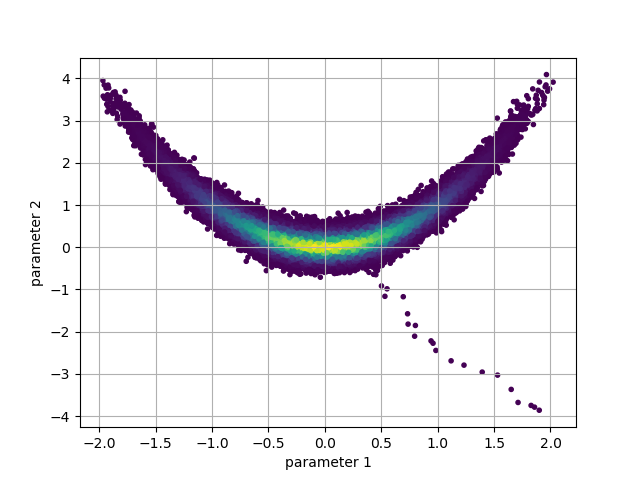
We can see from this plot that in order to take a representative sample, some early portion of the chain must be removed. This is referred to as the ‘burn-in’ period. This period allows the chain to both find the high density areas, and adjust the proposal widths to their optimal values.

The plot_diagnostics method can help us decide what size of burn-in to use:

chain.plot_diagnostics()

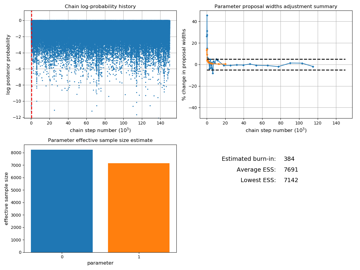
Occasionally samples are also ‘thinned’ by a factor of n (where only every n’th sample is used) in order to reduce the size of the data set for storage, or to produce uncorrelated samples.

Based on the diagnostics we can choose burn and thin values, which can be passed to methods of the chain that access or operate on the sample data.

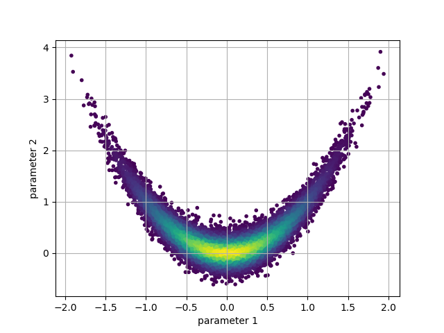
burn = 2000
thin = 10

By specifying the burn and thin values, we can generate a new version of the earlier plot with the burn-in and thinned samples discarded:

p = chain.get_probabilities(burn=burn, thin=thin)
pnt_colors = exp(p - p.max())
plt.scatter(
    chain.get_parameter(0, burn=burn, thin=thin),
    chain.get_parameter(1, burn=burn, thin=thin),
    c=pnt_colors,
    marker = '.'
)
plt.xlabel('parameter 1')
plt.ylabel('parameter 2')
plt.grid()
plt.show()

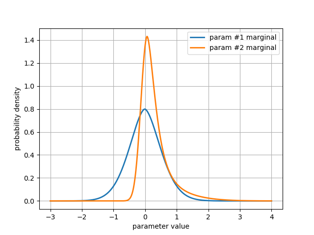
We can easily estimate 1D marginal distributions for any parameter using the get_marginal method:

pdf_1 = chain.get_marginal(0, burn=burn, thin=thin, unimodal=True)
pdf_2 = chain.get_marginal(1, burn=burn, thin=thin, unimodal=True)

get_marginal returns a density estimator object, which can be called as a function to return the value of the pdf at any point:

axis = linspace(-3, 4, 500) # axis on which to evaluate the marginal PDFs
# plot the marginal distributions
plt.plot(axis, pdf_1(axis), label='param #1 marginal', lw=2)
plt.plot(axis, pdf_2(axis), label='param #2 marginal', lw=2)
plt.xlabel('parameter value')
plt.ylabel('probability density')
plt.legend()
plt.grid()
plt.show()