HamiltonianChain

class inference.mcmc.HamiltonianChain(posterior: callable, start: ndarray, grad: callable = None, epsilon: float = 0.1, temperature: float = 1.0, bounds: Bounds = None, inverse_mass: ndarray = None, display_progress=True)

Class for performing Hamiltonian Monte-Carlo sampling.

Hamiltonian Monte-Carlo (HMC) is an MCMC algorithm where proposed steps are generated by integrating Hamilton’s equations, treating the negative posterior log-probability as a scalar potential. In order to do this, the algorithm requires the gradient of the log-posterior with respect to the model parameters. Assuming this gradient can be calculated efficiently, HMC deals well with strongly correlated variables and scales favourably to higher-dimensionality problems.

This implementation automatically selects an appropriate time-step for the Hamiltonian dynamics simulation, but currently does not dynamically select the number of time-steps per proposal, or appropriate inverse-mass values.

Parameters

posterior (func) – A function which takes the vector of model parameters as a numpy.ndarray, and returns the posterior log-probability.
start – Vector of model parameters which correspond to the parameter-space coordinates at which the chain will start.
grad (func) – A function which returns the gradient of the log-posterior probability density for a given set of model parameters theta. If this function is not given, the gradient will instead be estimated by finite difference.
epsilon (float) – Initial guess for the time-step of the Hamiltonian dynamics simulation.
temperature (float) – The temperature of the markov chain. This parameter is used for parallel tempering and should be otherwise left unspecified.
bounds – An instance of the inference.mcmc.Bounds class, or a sequence of two numpy.ndarray specifying the lower and upper bounds for the parameters in the form (lower_bounds, upper_bounds).
inverse_mass – A vector specifying the inverse-mass value to be used for each parameter. The inverse-mass is used to transform the momentum distribution in order to make the problem more isotropic. Ideally, the inverse-mass for each parameter should be set to the variance of the marginal distribution of that parameter.
display_progress (bool) – If set as True, a message is displayed during sampling showing the current progress and an estimated time until completion.

advance(m: int)

Advances the chain by taking m new steps.

Parameters: m (int) – Number of steps the chain will advance.

get_marginal(index: int, burn: int = 1, thin: int = 1, unimodal=False) → DensityEstimator

Estimate the 1D marginal distribution of a chosen parameter.

Parameters

index (int) – Index of the parameter for which the marginal distribution is to be estimated.
burn (int) – Number of samples to discard from the start of the chain.
thin (int) – Rather than using every sample which is not discarded as part of the burn-in, every m’th sample is used for a specified integer m.
unimodal (bool) – Selects the type of density estimation to be used. The default value is False, which causes a GaussianKDE object to be returned. If however the marginal distribution being estimated is known to be unimodal, setting unimodal = True will result in the UnimodalPdf class being used to estimate the density.

Returns

An instance of a DensityEstimator from the inference.pdf module which represents the 1D marginal distribution of the chosen parameter. If the unimodal argument is False a GaussianKDE instance is returned, else if True a UnimodalPdf instance is returned.

get_parameter(index: int, burn: int = 1, thin: int = 1) → ndarray

Return sample values for a chosen parameter.

Parameters

index (int) – Index of the parameter for which samples are to be returned.
burn (int) – Number of samples to discard from the start of the chain.
thin (int) – Instead of returning every sample which is not discarded as part of the burn-in, every m’th sample is returned for a specified integer m.

Returns

Samples for the parameter specified by index as a numpy.ndarray.

matrix_plot(params: list[int] = None, burn: int = 0, thin: int = 1, **kwargs)

Construct a ‘matrix plot’ of the parameters (or a subset) which displays all 1D and 2D marginal distributions. See the documentation of inference.plotting.matrix_plot for a description of other allowed keyword arguments.

Parameters

params – A list of integers specifying the indices of parameters which are to be plotted. If not specified, all parameters are plotted.
burn (int) – Sets the number of samples from the beginning of the chain which are ignored when generating the plot.
thin (int) – Sets the factor by which the sample is ‘thinned’ before generating the plot. If thin is set to some integer value m, then only every m’th sample is used, and the remainder are ignored.

plot_diagnostics(show=True, filename=None, burn=None)

Plot diagnostic traces that give information on how the chain is progressing.

Currently this method plots:

The posterior log-probability as a function of step number, which is useful for checking if the chain has reached a maximum. Any early parts of the chain where the probability is rising rapidly should be removed as burn-in.
The history of the simulation step-size epsilon as a function of number of total proposed jumps.
The estimated sample size (ESS) for every parameter, or in cases where the number of parameters is very large, a histogram of the ESS values.

Parameters

show (bool) – If set to True, the plot is displayed.
filename (str) – File path to which the diagnostics plot will be saved. If left unspecified the plot won’t be saved.

run_for(minutes=0, hours=0, days=0)

Advances the chain for a chosen amount of computation time.

Parameters

minutes (int) – number of minutes for which to run the chain.
hours (int) – number of hours for which to run the chain.
days (int) – number of days for which to run the chain.

trace_plot(params: list[int] = None, burn: int = 0, thin: int = 1, **kwargs)

Construct a ‘trace plot’ of the parameters (or a subset) which displays the value of the parameters as a function of step number in the chain. See the documentation of inference.plotting.trace_plot for a description of other allowed keyword arguments.

Parameters

params – A list of integers specifying the indices of parameters which are to be plotted. If not specified, all parameters are plotted.
burn (int) – Sets the number of samples from the beginning of the chain which are ignored when generating the plot.
thin (int) – Sets the factor by which the sample is ‘thinned’ before generating the plot. If thin is set to some integer value m, then only every m’th sample is used, and the remainder are ignored.

HamiltonianChain example code

Here we define a toroidal (donut-shaped!) posterior distribution which has strong non-linear correlation:

from numpy import array, sqrt

class ToroidalGaussian:
   def __init__(self):
      self.R0 = 1.  # torus major radius
      self.ar = 10. # torus aspect ratio
      self.inv_w2 = (self.ar / self.R0)**2

   def __call__(self, theta):
      x, y, z = theta
      r_sqr = z**2 + (sqrt(x**2 + y**2) - self.R0)**2
      return -0.5 * self.inv_w2 * r_sqr

   def gradient(self, theta):
      x, y, z = theta
      R = sqrt(x**2 + y**2)
      K = 1 - self.R0 / R
      g = array([K*x, K*y, z])
      return -g * self.inv_w2

Build the posterior and chain objects then generate the sample:

# create an instance of our posterior class
posterior = ToroidalGaussian()

# create the chain object
chain = HamiltonianChain(
    posterior = posterior,
    grad=posterior.gradient,
    start = [1, 0.1, 0.1]
)

# advance the chain to generate the sample
chain.advance(6000)

# choose how many samples will be thrown away from the start of the chain as 'burn-in'
burn = 2000

We can use the Plotly library to generate an interactive 3D scatterplot of our sample:

# extract sample and probability data from the chain
probs = chain.get_probabilities(burn=burn)
point_colors = exp(probs - probs.max())
x, y, z = [chain.get_parameter(i) for i in [0, 1, 2]]

# build the scatterplot using plotly
import plotly.graph_objects as go

fig = go.Figure(data=1[go.Scatter3d(
   x=x, y=y, z=z, mode='markers',
   marker=dict(size=5, color=point_colors, colorscale='Viridis', opacity=0.6)
)])

fig.update_layout(margin=dict(l=0, r=0, b=0, t=0)) # set a tight layout
fig.show()

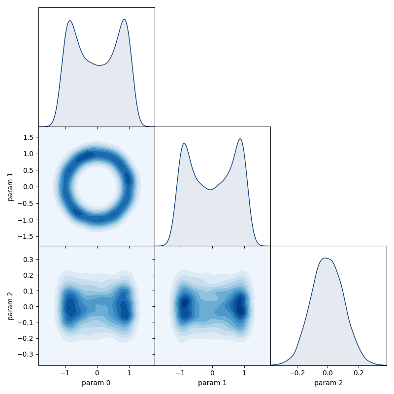
We can view all the corresponding 1D & 2D marginal distributions using the matrix_plot method of the chain:

chain.matrix_plot(burn=burn)